Immiscible color flows in optimal transport networks for image classification

1 Introduction

Optimal transport (OT) is a powerful method for computing the distance between two data distributions. This problem has a cross-disciplinary domain of applications, ranging from logistics and route optimization [1–3] to biology [4, 5] and computer vision [6–10], among others. Within this broad variety of problems, OT is largely utilized in machine learning [11] and deployed for solving classification tasks, where the goal is to optimally match discrete distributions that are typically learned from data. Relevant usage examples are also found in multiple fields of physics, as in protein fold recognition [12], stochastic thermodynamics [13], designing transportation networks [14, 15], routing in multilayer networks [16], or general relativity [17]. A prominent application is image classification [18–23], where the goal is to measure the similarity between two images. OT solves this problem by interpreting image pairs as two discrete distributions and then assessing their similarity via the Wasserstein (W₁) distance ([24], Definition 6.1), a measure obtained by minimizing the cost needed to transform one distribution into the other. Using W₁ for image classification carries many advantages over other similarity measures between histograms. For example, W₁ preserves all properties of a metric [9, 24], it is robust over domain shift for train and test data [22], and it provides meaningful gradients to learn data distributions on non-overlapping domains [25]. Because of these and several other desirable properties, much research effort has been put into speeding up algorithms to calculate W₁ [12, 19, 20, 26, 27]. However, all these methods overlook the potential of effectively using image colors directly in the OT formulation. As a result, practitioners have access to increasingly efficient algorithms, but those do not necessarily improve accuracy in predictions, as we lack a framework that fully exploits the richness of the input information.

Colored images originally encoded as three-dimensional histograms—with one dimension per color channel—are often compressed into lower dimensional data using feature extraction algorithms [9, 23]. Here, we propose a different approach that maps the three distinct color histograms to multicommodity flows transported in a network built using images’ pixels. We combine recent developments in OT with the physics insights of capacitated network models [1, 5, 28–31] to treat colors as masses of different types that flow through the edges of a network. Different flows are coupled together with a shared conductivity to minimize a unique cost function. This setup is reminiscent of the distinction between modeling the flow of one substance, e.g., water, and modeling the flows of multiple substances that do not mix, e.g., immiscible fluids, which share the same network infrastructure. By virtue of this multicommodity treatment, we achieve stronger classification performance than state-of-the-art OT-based algorithms in real datasets where color information matters.

2 Problem formulation

2.1 Unicommodity optimal transport

Given two m- and n-dimensional probability vectors g and h and a positive-valued ground cost matrix C, the goal of a standard—unicommodity—OT problem is to find an optimal transport path P^⋆ satisfying the conservation constraints ∑_jP_ij = g_i∀i and ∑_iP_ij = h_j∀j, while minimizing J(g, h) = ∑_ijP_ijC_ij.

Entries $P_{ij}^{\star }$ can be interpreted as the mass transported from g_i to h_j when paying a cost C_ij, while J^⋆, i.e., J evaluated at P^⋆, encodes the minimum effort needed to transport g to h. Notably, if all entries C_ij are distances between i and j, then J^⋆ is the W₁ distance between g and h (see [24] for a standard proof and [9] for derivations focusing on the discrete case).

2.2 Physics-inspired multicommodity optimal transport

Interpreting colors as masses traveling along a network built from images’ pixels (as we define in detail below), unicommodity OT could be used to capture the similarity between grayscale images. However, it may not be ideal for colored images, when color information matters. The limitation of unicommodity OT in Section 2.1 is that it does not fully capture the variety of information contained in different color channels as it is not able to distinguish them. Motivated by this, we tackle this challenge and move beyond this standard setting by incorporating insights from the dynamics of immiscible flows into physics. Specifically, we treat the different pixels’ color channels as masses of different types that do not mix but rather travel and interact on the same network infrastructure, while optimizing a unique cost function. By assuming capacitated edges with conductivities that are proportional to the amount of mass traveling through an edge, we can define a set of ODEs that regulate fluxes and conductivities. These are optimally distributed along a network to better account for color information while satisfying physical conservation laws. Similar ideas have been successfully used to route different types of passengers in transportation networks [2, 16, 32].

Formally, we couple together the histograms of M = 3 color channels, the commodities, indexed with a = 1, …, M. We define g^a and h^a as m- and n-dimensional probability vectors of mass of type a. More compactly, we define the matrix G with entries $G_{ia}=g_i^a$ (respectively, H for h), each containing the intensity of color channel a in pixel i of the first (respectively, second) image. These regulate the sources and sinks of mass in our setting. We then enforce the conservation of mass for each commodity index a ${\sum }_i{g}_i^a={\sum }_j{h}_j^a$. This ensures that all the color mass in the first image is accounted for in the second image, and vice versa. This should be valid for each mass type.

Moreover, we define the set Π(G, H) containing (m × n × M)-dimensional tensors P with entries $P_{ij}^a$ being transport paths between g^a and h^a. These regulate how fluxes of colors of different types travel along a network. We enforce the interaction between transport paths for different commodities by introducing a shared cost.

where $\Vert P_{ij}{\Vert }_2={({\sum }_a{P_{ij}^a}^2)}^{1/2}$ is the 2-norm of the vector $P_{ij}=\left(P_{ij}^1,\dots ,P_{ij}^M\right)$ and 0 < Γ < 4/3 is a regularization parameter. We take Γ > 0 since a negative exponent would favor the proliferation of loops with infinite mass [28]. Instead, we conventionally consider Γ < 4/3 (see Section 3.2) since the cost J_Γ exhibits the same convexity properties for any Γ > 1, i.e., it is strictly convex, and OT paths do not change substantially with Γ in this regime [2]. We can thus formulate its corresponding multicommodity OT problem as that of finding a tensor P^⋆ solution of

It should be noted that for M = 1 and Γ = 1, we recover the standard unicommodity OT setup.

The problem in Eq. 2 admits a precise physical interpretation. In fact, it can be recast as a constrained minimization problem with the objective function being the energy dissipated by the multicommodity flows (Joule’s law) and a constant total conductivity. Furthermore, transport paths follow Kirchhoff’s law enforcing conservation of mass [2, 32, 33] (see Supplementary Material for a detailed discussion).

Noticeably, J_Γ is a quantity that takes into account all the different mass types, and the OT paths P^⋆ are found through a unique optimization problem. We emphasize that this is fundamentally different from solving M-independent unicommodity problems, where different types of mass are not coupled together as in our setting, and then combining their optimal costs to estimate images’ similarity. Estimating $J_{\mathrm{\Gamma }}^{\star }(G,H)$ directly gives a quantitative and principled measure of the similarity between two images G and H. The lower this cost, the higher the similarity of the two images. While this is valid also for the unicommodity cost in Section 2.1, the difference here is that we account differently for the color information as we distinguish different colors via the M-dimensional vector P_ij. The cost in Eq. 2 then properly couples colors by following physical laws regulating immiscible flows. The idea is that if this information matters for the given classification task, incorporating it into the minimization problem would output a cost that helps to distinguish images better, e.g., with higher accuracy.

3 Materials and methods

3.1 Optimal transport network on images

Having introduced the main ideas and intuitions, we now explain in detail how to adapt the OT formalism to images. Specifically, we introduce an auxiliary bipartite network K_m,n(V₁, V₂, E₁₂), which is the first building block of the network where the OT problem is solved. A visual representation of this is shown in Figure 1. The images 1 and 2 are represented as matrices (G and H) of sizes m × M and n × M, respectively, where M is the number of color channels of the images (M = 3 in our examples). The sets of nodes V₁ and V₂ of the network K_m,n are the pixels of images 1 and 2, respectively. The set of edges E₁₂ contains a subset of all pixel pairs between the two images, as detailed further. We consider the cost of an edge (i, j) as

where the vector v_i = (x_i, y_i) contains the horizontal and vertical coordinates of pixel i of image 1 (similarly v_j for image 2). The quantity θ ∈ [0, 1] is a hyperparameter that is given in input and can be chosen with cross-validation. It acts as a weight for a convex combination between the Euclidean distance between pixels and the difference in their color intensities, following the intuition in [9, 23]. When θ = 0, the OT path P^⋆ is the one that minimizes only the geometrical distance between pixels. Instead, when θ = 1, pixels’ locations are no longer considered, and transport paths are only weighted by color distributions. The parameter τ is introduced following [22, 23] with the scope of removing all edges with cost C_ij(θ, τ) = τ, i.e., those for which (1 − θ)‖v_i − v_j‖₂ + θ‖G_i − H_j‖₁ > τ. These are substituted by m + n transshipment edges e ∈ E′, each of which has a cost of τ/2 and is connected to one unique auxiliary vertex u₁. Thresholding the cost decreases significantly the computational complexity of OT, making it linear with the number of nodes |V₁| + |V₂| + 2 = m + n + 2 (see Supplementary Material).

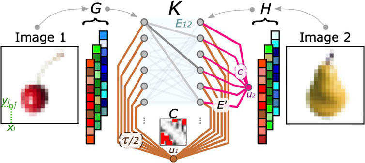
FIGURE 1. Bipartite network representation for multicommodity OT. The two images (shown on the leftmost and rightmost sides of the panel) are encoded in the RGB matrices G and H, which regulate the flow traveling on the network K. The graph is made of m + n + 2 nodes, i.e., the total number of pixels plus the two auxiliary vertices introduced in Section 3.1. Gray edges (belonging to the set E₁₂) connect nodes in image 1 to nodes in image 2; these edges are trimmed according to a threshold τ. We highlight the entries of the matrix C in red if these are larger than τ. Transshipment and auxiliary edges used to relax mass conservation (which belong to E′) are colored in brown and magenta.

Furthermore, we relax the conservation of mass by allowing ∑_iG_ia ≠ ∑_jH_ja. The excess mass m^a = ∑_jH_ja − ∑_iG_ia is assigned to a second auxiliary node, u₂. We connect it to the network with n additional transshipment edges, e ∈ E′, each penalizing the total cost by c = max_ijC_ij/2. This construction improves classification when the histograms’ total masses largely differ [22]. Intuitively, this can happen when comparing “darker” images against “brighter” images more precisely, when entries of g^a and h^a are further apart in the RGB color space.

Overall, we obtain a network K with nodes $V=V_1\cup V_2\cup \left\{u_1,u_2\right\}$ and edges E = E₁₂ ∪ E′, i.e., the original bipartite graph K_m,n, together with the auxiliary transshipment links and nodes. It should be noted that in its entirety, the system is isolated, i.e., the total mass is conserved. See Supplementary Material for a detailed description of the OT setup.

Given this auxiliary graph, the OT problem is then solved by injecting the color mass contained in image 1 in nodes i ∈ V₁, as specified by G, and extracting it from nodes j ∈ V₂ of image 2, as specified by H. This is carried out by transporting mass using either i) an edge in E₁₂ or ii) a transshipment one in E′. In the following section, we describe how this problem is solved mathematically.

3.2 Optimizing immiscible color flows: The dynamics

We solve the OT problem by proposing the following ODEs for controlling mass transportation:

which constitute the pivotal equations of our model. Here, we introduce the shared conductivities x_e ≥ 0 and define $S_i^a=G_{ia}-H_{ia}$, taking values $S_{u_1}^a=0$ and $S_{u_2}^a=m^a$ on the auxiliary nodes. With L_ij[x] = ∑_e(x_e/C_e)B_ieB_je, we denote the weighted Laplacian of K, where B is its signed incidence matrix and ∂i is the neighborhood of node i. Lastly, ${\varphi }_i^a$ is the scalar potential acting on nodes for a given commodity a. The least-square solutions of Eq. 4 are ${\varphi }_i^a[x]={\sum }_j{L}_{ij}^{†}[x]S_i^a$, where † denotes the Moore–Penrose inverse. The critical exponent 0 < β < 2 [Γ = 2(2 − β)/(3 − β)] is a hyperparameter that needs to be chosen before solving Eqs 4 and 5. Depending on the modeling task, its value can be fixed a priori (e.g., β = 1 for the shortest path problem [34], β ≃ 5/3 for river networks [35], and β → 2⁻ for the Steiner tree problem [36]) or cross-validated as we do here for image classification. The exponent aggregates paths using the principle of economy of scale if 1 < β < 2. It dilutes them along the network otherwise, with the goal of reducing traffic congestion. This behavior is a direct consequence of the subadditivity of J_Γ in Eq. 2 for β > 1 (Γ < 1), and, respectively, superadditivity for β < 1 (Γ > 1). It has been theoretically discussed and empirically observed, for example, in [32, 37, 38].

The feedback mechanism of Eq. 5 defines multicommodity fluxes $(P_e^a)$ that are admissible for the minimization problem introduced in Eq. 2. Particularly, for color of type a on edges e = (i, j), we couple potentials $({\varphi }_i^a)$ that are the solutions of Eq. 4 and shared conductivities (x_e) to define

This also highlights another physical interpretation; i.e., by interpreting the ${\varphi }_i^a$ as pressure potentials, the fluxes are seen to arise from a difference in pressure between two nodes as in hydraulic or electrical networks. Crucially, this allocation is governed by one unique conductivity for all commodities, whose dynamics depends on the 2-norm over a of differences in potentials, as in Eq. 5. In analogy with immiscible flows, this ensures that flows of different types share the same infrastructure, and in practice, it couples them into a unique optimization problem.

In the case of only one commodity (M = 1), variants of this dynamics have been used to model transport optimization in various physical systems [1, 5, 29–31].

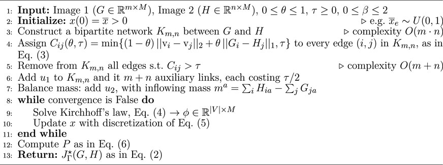
The salient result of our construction is that the asymptotic trajectories of Eqs 4 and 5 are equivalent to the minimizers of Eq. 2, i.e., lim_t→+∞P(t) = P^⋆ (see Supplementary Material for derivations following [32, 33]). Therefore, numerically integrating our dynamics solves the multicommodity OT problem. In other words, this allows us to estimate the optimal cost in Eq. 2 and use that to compute similarities between images. A pseudo-code of the algorithmic implementation is shown in Algorithm 1.

Algorithm 1. Multicommodity dynamics.

3.3 Computational complexity

In principle, our multicommodity method has a computational complexity of order O(M|V|²) for complete transport network topologies, i.e., when edges in the transport network K are assigned to all pixel pairs. Nonetheless, we substantially reduce this complexity to O(M|V|) by sparsifying the graph with the trimming procedure of [22, 23]. More details are given in Supplementary Material. Empirically, we observe that by running Eqs 4 and 5, most of the entries of x decay to zero after a few steps, producing a progressively sparser weighted Laplacian L[x]. This allows for faster computation of the Moore–Penrose inverse L^†[x] and least-square potentials ${\varphi }_i^a={\sum }_j{L}_{ij}^{†}[x]S_j^a$. A thorough experimental analysis of the convergence properties of the OT dynamics has been carried out in [39].

4 Results and discussion

4.1 Classification task

We provide empirical evidence that our multicommodity dynamics outperforms competing OT algorithms on classification tasks. As anticipated previously, we use the OT optimal cost $J_{\mathrm{\Gamma }}^{\star }$ as a measure of similarity between two images and perform supervised classification with a k-nearest neighbor (k-NN) classifier as described in [20]. Alternative methods (e.g., SVM as in [19]) could also be used for this task. However, these may require the cost $J_{\mathrm{\Gamma }}^{\star }$ to satisfy the distance axioms to properly induce a kernel. While it is not straightforward to verify these conditions for the OT cost in Eq. 2, this is not necessary for the k-NN classifier, which requires looser conditions on $J_{\mathrm{\Gamma }}^{\star }$.

We compare the classification accuracy of our model against i) the Sinkhorn algorithm [19, 40] (utilizing the more stable Sinkhorn scheme proposed in [41]); ii) a unicommodity dynamics executed on grayscale images, i.e., with color information compressed into one single commodity (M = 1); and iii) the Sinkhorn algorithm on grayscale images. All methods are tested on the following two datasets: the Jena Flowers 30 Dataset (JF30) [42] and the Fruit Dataset (FD) [43]. The first consists of 1,479 images of 30 wild-flowering angiosperms (flowers). Flowers are labeled with their species, and inferring them is the goal of the classification task. The second dataset contains 15 fruit types and 163 images. Here, we want to classify fruit types. The parameters of the OT problem setup (θ and τ) and regularization parameters (β and ɛ, which enforce the entropic barrier in the Sinkhorn algorithm [19]), have been cross-validated for both datasets (see Section 3 and Section 4 in Supplementary Material). All methods are then tested in their optimal configurations (see Supplementary Material for implementation details).

Classification results are shown in Table 1. In all cases, leveraging colors leads to higher accuracy (about an 8% increase) with respect to classification performed using grayscale images. This signals that in the datasets under consideration, color information is a relevant feature for differentiating image samples. Remarkably, we get a similar increase in performance (about 7%–8%) on both colored datasets when comparing our multicommodity dynamics against the Sinkhorn algorithm. As the two algorithms use the same (colored) input, we can attribute this increment to the effective usage of color that our approach is capable of.

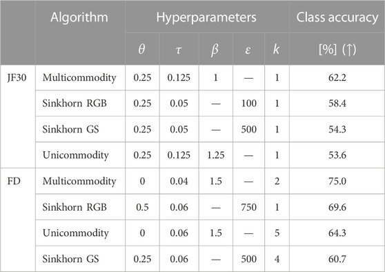
TABLE 1. Classification task results. With multicommodity, Sinkhorn RGB, unicommodity, and Sinkhorn GS, we label methods on colored images (the first two) and grayscale images (the second two). The optimal parameters in the central columns are selected with a 4-fold cross-validation; k is the number of nearest neighbors used in the classifier. The rightmost column shows the fraction (in percentage) of correctly classified images. Results are ordered by performance, and we highlight the best ones in bold.

In addition, by analyzing results in more detail, we first observe that on JF30, all methods perform best when θ = 0.25, i.e., 25% of the information used to build C comes from colors. This trend does not recur on the FD, where both dynamics favor θ = 0 (Euclidean C). Hence, our model is able to leverage color information via the multicommodity OT dynamical formulation.

Second, on JF30, both dynamics perform best with τ = 0.125, contrary to Sinkhorn-based methods that prefer τ = 0.05. Thus, Sinkhorn’s classification accuracy is negatively affected both by low τ—many edges of the transport network are cut—and by large τ —noisy color information is used to build C. We do not observe this behavior in our model, where trimming fewer edges is advantageous. All optimal values of τ are lower on the FD since the color distributions in this dataset are naturally light-tailed (see Supplementary Material).

Lastly, we investigate the interplay between θ and β. We notice that θ = 0 (FD) corresponds to higher β = 1.5. Instead, for larger θ = 0.25 (JF30), the model prefers lower β (β = 1 and 1.25 for the multicommodity and unicommodity dynamics, respectively). In the former case (θ = 0, C_ij is the Euclidean distance), the cost is equal to zero for pixels with the same locations. Thus, consolidation of transport paths—large β—is favored on cheap links. Instead, increasing θ leads to more edges with comparable costs as colors distribute smoothly over images. In this second scenario, better performance is achieved with distributed transport paths, i.e., lower β (see Supplementary Material).

4.2 Performance in terms of sensitivity

We assess the effectiveness of our method against benchmarks by comparing the sensitivity of our multicommodity dynamics and that of the Sinkhorn algorithm on the colored JF30 dataset. Specifically, we set all algorithm parameters to their best configurations, as shown in Table 1. Then, for each of the 30 classes in JF30, we compute its one-to-all sensitivity, i.e., the true positive rate. This is defined for any class c as

where TP(c) is the true positive rate, i.e., the number of images in c that are correctly classified; FN(c) is the false negative rate, i.e., the number of c-samples that are assigned a label different from c. Hence, Eq. 7 returns the probability that a sample is assigned label c, given that it belongs to c.

We find that our method robustly outperforms the Sinkhorn algorithm. Specifically, the multicommodity dynamics has the highest sensitivity 50% of the times—15 classes out of a total of 30—as shown in Figure 2. For nine classes, Sinkhorn has higher sensitivity, and for six classes, both methods give the same values of S.Furthermore, we find that in 2/3 (20 out of 30) of the classes, the multicommodity dynamics returns S(c) ≥ 1/2. This means that our model predicts the correct label more than 50% of the time. In only three out of these 20 cases, Sinkhorn attains higher values of S, while in most instances where Sinkhorn outperforms our method, it has a lower sensitivity of S < 1/2. Hence, this is the case in classes where both methods have difficulty distinguishing images.

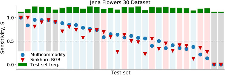
FIGURE 2. Sensitivity on the JF30 dataset. Sensitivity values are shown for the multicommodity dynamics (blue circles) and for Sinkhorn RGB (red triangles). Markers are sorted in descending order of S, regardless of the method. Background colors are blue, red, and gray, when S is higher for the multicommodity method, the Sinkhorn algorithm, or none of them, respectively. In green, we plot frequency bars for all classes in the test set.

4.3 The impact of colors

To further assess the significance of leveraging color information, we conduct three different experiments that highlight both qualitatively and quantitatively various performance differences between the unicommodity and multicommodity approaches. As the two share the same principled dynamics based on OT with the main difference being that multicommodity does not compress the color information, we can use this analysis to better understand how fully exploiting the color information drives better classification.

Experiment 1: Landscape of optimal cost. Here, we focus on a qualitative comparison between the cost landscapes obtained with the two approaches. We consider the example of an individual image taken from the FD test set and plot the landscape of optimal costs $J_{\mathrm{\Gamma }}^{\star }$ when comparing it to the train set. Results for the multicommodity dynamics (M = 3) and the unicommodity dynamics (M = 1) on grayscale images are shown in Figure 3. Here, we highlight the five lowest values of the cost and mark them in green if they correspond to correctly classified train samples and in red otherwise. At first glance, one may conclude that their performance is identical (as both dynamics classify correctly three samples out of five), and we notice how the multicommodity dynamics consistently clusters them at the bottom of the cost landscape, thus ranking them in a better order. This may explain why the cross-validated best value of k (the number of nearest neighbors in the k-NN classifier) is higher for unicommodity methods in this dataset. On a larger sample of data, this results in better overall classification performance, as shown in Table 1.

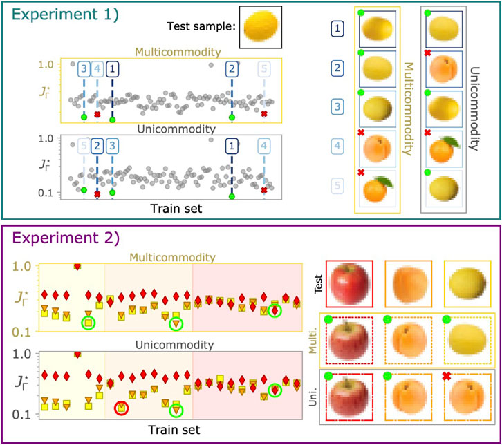
FIGURE 3. Evaluating the effect of colors. Experiment 1: The top black-framed image is the one to be classified. Predictions given by the multicommodity and unicommodity dynamics (those with lower $J_{\mathrm{\Gamma }}^{\star }$) are shown on the right side of the panel and are displayed in a sorted fashion from worst to best (from bottom to top). Experiment 2: The top right samples are the three test images to be classified. Middle and bottom rows are predictions given by the two dynamics. Markers, backgrounds, and test images shared a color code: red for apples, orange for apricots, and yellow for melons. In both panels, green circles and red crosses are used to highlight classified and misclassified images, respectively. All algorithms are executed with their optimal configurations listed in Table 1.

Experiment 2: Controlling for shape. We further mark this tendency with a second experiment where we select a subset of the FD composed of images belonging to three classes of fruits that have similar shapes but different colors such as red apples, orange apricots, and yellow melons. As we expect shape to be less informative than colors in this custom set, we can assess the extent to which color plays a crucial role in the classification process. Specifically, the test set is made of three random samples, each drawn from one of these classes (top row of the rightmost panel) in Figure 3, while the train set contains the remaining instances of the classes. We plot the cost landscape $J_{\mathrm{\Gamma }}^{\star }$ for the train set and draw in the red, orange, and yellow values of $J_{\mathrm{\Gamma }}^{\star }$ that correspond to the samples that are compared against the test apple, apricot, and melon, respectively. We also sort the train samples so that they are grouped in three regions (highlighted by the background color in Figure 3), which correspond to train melons, apricots, and apples. With this construction, if the minimum cost among the yellow markers falls in the yellow region, it will correspond to a correctly classified sample (respectively, for orange and red). We further mark the yellow, orange, and red minima in green if the test and train labels correspond, i.e., the marker’s and background colors are the same, and in red otherwise. Train and test samples are also in Figure 3. The multicommodity dynamics correctly label each test image. In contrast, unicommodity dynamics fails at this task, labeling a melon as an apricot. This suggests that the multicommodity approach is able to use the color information in datasets where this feature is more informative than others, e.g., shape.

Experiment 3: When shape matters. Having shown results on a custom dataset where shape was controlled to matter less, we now do the opposite and select a dataset where this feature should be more informative. The goal is to assess whether a multicommodity approach helps in this case as well, as its main input information may not be as relevant anymore. Specifically, we select as a test sample a cherry, whose form is arguably distinguishable from that of many other fruits in the dataset. One can expect that comparing it against the train set of the FD will result in having both unicommodity and multicommodity dynamics able to assign low $J_{\mathrm{\Gamma }}^{\star }$ to train cherries and higher costs to other fruits. This intuition is confirmed by the results in Figure 4. Here, train cherries (in green) strongly cluster in the lower portion of the cost landscape, whereas all the other fruits have higher costs. In Figure 4, we also plot some of the correctly classified train samples. These results suggest that when color information is negligible compared to another type of information (e.g., shape), unicommodity and multicommodity formulations perform similarly. In light of this, we reinforce the claim that our multicommodity formulation can boost classification in contexts where color information does matter but may not give any advantage when other types of information are more informative. We encourage practitioners to evaluate when this is the case based on domain knowledge when available.

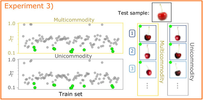
FIGURE 4. Evaluating the importance of colors: when shapes matter most. Experiment 3: The top black-framed image is the one to be classified. The best three (out of 10) predictions returned by the two dynamics are shown on the right. We mark the training samples belonging to the same class as the test image with green circles. All algorithms are executed with their optimal configurations listed in Table 1.

5 Conclusion

We propose a physics-informed multicommodity OT formulation for effectively using color information to improve image classification. We model colors as immiscible flows traveling on a capacitated network and propose equations for its dynamics, with the goal of optimizing flow distribution on edges. Color flows are regulated by a shared conductivity to minimize a unique cost function. Thresholding the ground cost as in [22, 23] makes our model computationally efficient.

We outperform other OT-based approaches such as the Sinkhorn algorithm on two datasets where color matters. Our model also assigns a lower cost to correctly classified images than its unicommodity counterpart, and it is more robust on datasets where items have similar shape. Thus, color information is distinctly relevant. We note that for some datasets, color information may not matter as much as another type of information (e.g., shape), which has stronger discriminative power. However, while we focused here on different color channels as the different commodities in our formulation, the ideas of this study can be extended to scenarios where other relevant information can be distinguished into different types. For instance, one could combine several features together, e.g., colors, contours, and objects’ orientations when available.

Our model can be further improved. While it uses the thresholding of [22, 23] to speed up convergence (as mentioned in Section 3.1), it is still slower than Sinkhorn-based methods. Hence, investigating approaches aimed at improving its computational performance is an important direction for future work. Speed-up can be achieved, for example, with the implementation of [39], where the unicommodity OT problem on sparse topologies is solved in O(|E|^0.36) time steps. This bound has been found using a backward Euler scheme combined with the inexact Newton–Raphson method for the update of x and solving Kirchhoff’s law using an algebraic multigrid method [44].

Our main goal is to frame an image classification task into that of finding optimal flows of masses of different types in networks built from images. We follow physics principles to assess whether using colors as immiscible flows can give an advantage compared to other standard OT-based methods that do not incorporate such insights. The increased classification performance observed in our experiments stimulates the integration of similar ideas into deep network architectures [45] as a relevant avenue for future work. Combining their prediction capabilities with our insights on how to better exploit the various facets of the input data has the potential to push the performance of deep classifiers even further. For example, one could extend the state-of-the-art architecture of Eisenberger et al. [45], which efficiently computes implicit gradients for generic Sinkhorn layers within a neural network, by including edge, shape, and contour information for Wasserstein barycenter computation or image clustering.

Data availability statement

The original contributions presented in the study are publicly available. This data can be found here: https://doi.org/10.7910/DVN/QDHYST, https://github.com/daniloeler/fruitdataset.

Author contributions

All authors contributed to developing the models, conceiving the experiments, analyzing the results, and reviewing the manuscript. AL and DB conducted the experiments. All authors read and agreed to the published version of the manuscript.

Acknowledgments

The authors thank the International Max Planck Research School for Intelligent Systems (IMPRS-IS) for supporting AL and DB.

Conflict of interest

The authors declare that the research was conducted in the absence of any commercial or financial relationships that could be construed as a potential conflict of interest.

Publisher’s note

All claims expressed in this article are solely those of the authors and do not necessarily represent those of their affiliated organizations, or those of the publisher, the editors, and the reviewers. Any product that may be evaluated in this article, or claim that may be made by its manufacturer, is not guaranteed or endorsed by the publisher.

Supplementary material

The Supplementary Material for this article can be found online at: https://www.frontiersin.org/articles/10.3389/fphy.2023.1089114/full#supplementary-material

References

1. Kaiser F, Ronellenfitsch H, Witthaut D. Discontinuous transition to loop formation in optimal supply networks. Nat Commun (2020) 11:5796–11. doi:10.1038/s41467-020-19567-2
2. Lonardi A, Putti M, De Bacco C. Multicommodity routing optimization for engineering networks. Scientific Rep (2022) 12:7474. doi:10.1038/s41598-022-11348-9
3. Lonardi A, Facca E, Putti M, De Bacco C. Infrastructure adaptation and emergence of loops in network routing with time-dependent loads. arXiv (2021). doi:10.48550/ARXIV.2112.10620
4. Demetci P, Santorella R, Sandstede B, Noble WS, Singh R. Gromov-Wasserstein optimal transport to align single-cell multi-omics data. bioRxiv (2020). doi:10.1101/2020.04.28.066787
5. Katifori E, Szöllősi GJ, Magnasco MO. Damage and fluctuations induce loops in optimal transport networks. Phys Rev Lett (2010) 104:048704. doi:10.1103/PhysRevLett.104.048704
6. Werman M, Peleg S, Rosenfeld A. A distance metric for multidimensional histograms. Comput Vis Graphics, Image Process (1985) 32:328–36. doi:10.1016/0734-189X(85)90055-6
7. Peleg S, Werman M, Rom H. A unified approach to the change of resolution: Space and gray-level. IEEE Trans Pattern Anal Machine Intelligence (1989) 11:739–42. doi:10.1109/34.192468
8. Rubner Y, Tomasi C, Guibas LJ. A metric for distributions with applications to image databases. In: Sixth International Conference on Computer Vision (IEEE Cat. No.98CH36271). Bombay, India: IEEE (1998). p. 59–66. doi:10.1109/ICCV.1998.710701
9. Rubner Y, Tomasi C, Guibas LJ. The earth mover’s distance as a metric for image retrieval. Int J Comput Vis (2000) 40:99–121. doi:10.1023/A:1026543900054
10. Baptista D, De Bacco C. Principled network extraction from images. R Soc Open Sci (2021) 8:210025. doi:10.1098/rsos.210025
11. Peyré G, Cuturi M. Computational optimal transport: With applications to data science. Foundations Trends® Machine Learn (2019) 11:355–607. doi:10.1561/2200000073
12. Koehl P, Delarue M, Orland H. Optimal transport at finite temperature. Phys Rev E (2019) 100:013310. doi:10.1103/PhysRevE.100.013310
13. Aurell E, Mejía-Monasterio C, Muratore-Ginanneschi P. Optimal protocols and optimal transport in stochastic thermodynamics. Phys Rev Lett (2011) 106:250601. doi:10.1103/PhysRevLett.106.250601
14. Leite D, De Bacco C. Revealing the similarity between urban transportation networks and optimal transport-based infrastructures. arXiv preprint arXiv:2209.06751 (2022).
15. Baptista D, Leite D, Facca E, Putti M, De Bacco C. Network extraction by routing optimization. Scientific Rep (2020) 10:20806. doi:10.1038/s41598-020-77064-4
16. Ibrahim AA, Lonardi A, Bacco CD. Optimal transport in multilayer networks for traffic flow optimization. Algorithms (2021) 14:189. doi:10.3390/a14070189
17. Mondino A, Suhr S. An optimal transport formulation of the Einstein equations of general relativity. J Eur Math Soc (2022). doi:10.4171/JEMS/1188
18. Grauman K, Darrell T. Fast contour matching using approximate Earth mover’s distance. In: Proceedings of the 2004 IEEE Computer Society Conference on Computer Vision and Pattern Recognition, 2004. CVPR 2004; 27 June 2004 - 02 July 2004. Washington, DC, USA: IEEE (2004). doi:10.1109/CVPR.2004.1315035
19. Cuturi M. Sinkhorn distances: Lightspeed computation of optimal transport. In: Advances in neural information processing systems, Vol. 26. Red Hook, NY, USA: Curran Associates, Inc. (2013). p. 2292–300.
20. Koehl P, Delarue M, Orland H. Statistical physics approach to the optimal transport problem. Phys Rev Lett (2019) 123:040603. doi:10.1103/PhysRevLett.123.040603
21. Thorpe M, Park S, Kolouri S, Rohde GK, Slepčev D. A transportation Lp distance for signal analysis. J Math Imaging Vis (2017) 59:187–210. doi:10.1007/s10851-017-0726-4
22. Pele O, Werman M. A linear time histogram metric for improved SIFT matching. In: Computer vision – ECCV 2008. Berlin, Heidelberg: Springer Berlin Heidelberg (2008). p. 495–508. doi:10.1007/978-3-540-88690-7_37
23. Pele O, Werman M. Fast and robust earth mover’s distances. In: 2009 IEEE 12th International Conference on Computer Vision. Kyoto, Japan: IEEE (2009). p. 460–7. doi:10.1109/ICCV.2009.5459199
24. Villani C. In: Optimal transport: Old and new, Vol. 338. Berlin, Heidelberg: Springer (2009). doi:10.1007/978-3-540-71050-9
25. Arjovsky M, Chintala S, Bottou L. Wasserstein generative adversarial networks. In: D Precup, and YW Teh, editors. Proceedings of the 34th international conference on machine learning (PMLR). Proceedings of machine learning research, Vol. 70 (2017). p. 214–23.
26. Lin T, Ho N, Jordan M. On efficient optimal transport: An analysis of greedy and accelerated mirror descent algorithms. In: Proceedings of the 36th international conference on machine learning (PMLR). In: Proceedings of machine learning research, Vol. 97 (2019). p. 3982–91.
27. Dvurechensky P, Gasnikov A, Kroshnin A. Computational optimal transport: Complexity by accelerated gradient descent is better than by Sinkhorn’s algorithm. In: Proceedings of the 35th international conference on machine learning (PMLR). In: Proceedings of machine learning research, Vol. 80 (2018). p. 1367–76.
28. Banavar JR, Colaiori F, Flammini A, Maritan A, Rinaldo A. Topology of the fittest transportation network. Phys Rev Lett (2000) 84:4745–8. doi:10.1103/PhysRevLett.84.4745
29. Ronellenfitsch H, Katifori E. Global optimization, local adaptation, and the role of growth in distribution networks. Phys Rev Lett (2016) 117:138301. doi:10.1103/PhysRevLett.117.138301
30. Hu D, Cai D. Adaptation and optimization of biological transport networks. Phys Rev Lett (2013) 111:138701. doi:10.1103/PhysRevLett.111.138701
31. Corson F. Fluctuations and redundancy in optimal transport networks. Phys Rev Lett (2010) 104:048703. doi:10.1103/PhysRevLett.104.048703
32. Lonardi A, Facca E, Putti M, De Bacco C. Designing optimal networks for multicommodity transport problem. Phys Rev Res (2021) 3:043010. doi:10.1103/PhysRevResearch.3.043010
33. Bonifaci V, Facca E, Folz F, Karrenbauer A, Kolev P, Mehlhorn K, et al. Physarum-inspired multi-commodity flow dynamics. Theor Comput Sci (2022) 920:1–20. doi:10.1016/j.tcs.2022.02.001
34. Bonifaci V, Mehlhorn K, Varma G. Physarum can compute shortest paths. J Theor Biol (2012) 309:121–33. doi:10.1016/j.jtbi.2012.06.017
35. Rinaldo A, Rodriguez-Iturbe I, Rigon R, Ijjasz-Vasquez E, Bras RL. Self-organized fractal river networks. Phys Rev Lett (1993) 70:822–5. doi:10.1103/PhysRevLett.70.822
36. Barabási AL. Invasion percolation and global optimization. Phys Rev Lett (1996) 76:3750–3. doi:10.1103/PhysRevLett.76.3750
37. Santambrogio F. Optimal channel networks, landscape function and branched transport. Inter Free Boundaries (2007) 9:149–69. doi:10.4171/IFB/160
38. Ibrahim AA, Leite D, De Bacco C. Sustainable optimal transport in multilayer networks. Phys Rev E (2022) 105:064302. doi:10.1103/PhysRevE.105.064302
39. Facca E, Benzi M. Fast iterative solution of the optimal transport problem on graphs. SIAM J Scientific Comput (2021) 43:A2295–A2319. doi:10.1137/20M137015X
40. Flamary R, Courty N, Gramfort A, Alaya MZ, Boisbunon A, Chambon S, et al. POT: Python optimal transport. J Machine Learn Res (2021) 22:1–8.
41. Schmitzer B. Stabilized sparse scaling algorithms for entropy regularized transport problems. SIAM J Scientific Comput (2019) 41:A1443–A1481. doi:10.1137/16M1106018
42. Seeland M, Rzanny M, Alaqraa N, Wäldchen J, Mäder P. Jena Flowers 30 dataset (2017). doi:10.7910/DVN/QDHYST
43. Macanhã PA, Eler DM, Garcia RE, Junior WEM. Handwritten feature descriptor methods applied to fruit classification. In: Information Technology - new generations. Cham: Springer International Publishing (2018). p. 699–705. doi:10.1007/978-3-319-54978-1_87
45. Eisenberger M, Toker A, Leal-Taixé L, Bernard F, Cremers D. A unified framework for implicit sinkhorn differentiation. In: Proceedings of the IEEE/CVF Conference on Computer Vision and Pattern Recognition (CVPR) (2022). p. 509–18.
46.MODI (Open Source code implementation) (2022). Available from: https://github.com/aleable/MODI.
Keywords: network flow optimization, image classification, network optimization, optimal transport, self-adapting dynamical systems
Citation: Lonardi A, Baptista D and De Bacco C (2023) Immiscible color flows in optimal transport networks for image classification. Front. Phys. 11:1089114. doi: 10.3389/fphy.2023.1089114
Received: 03 November 2022; Accepted: 20 January 2023;
Published: 27 February 2023.
Edited by:
Adriano Tiribocchi, National Research Council (CNR), ItalyReviewed by:
Giovanni Franzina, Istituto per le Applicazioni del Calcolo (IAC), ItalyPablo Villegas, Enrico Fermi Center for Study and Research, Italy
Copyright © 2023 Lonardi, Baptista and De Bacco. This is an open-access article distributed under the terms of the Creative Commons Attribution License (CC BY). The use, distribution or reproduction in other forums is permitted, provided the original author(s) and the copyright owner(s) are credited and that the original publication in this journal is cited, in accordance with accepted academic practice. No use, distribution or reproduction is permitted which does not comply with these terms.
*Correspondence: Alessandro Lonardi, alessandro.lonardi@tuebingen.mpg.de; Diego Baptista, diego.theuerkauf@tuebingen.mpg.de
†These authors have contributed equally to this work and share first authorship